Examples

Here we present a set of very simple examples just for you to get a feeling about the package.

Hello World

Consider the mighty Bernoulli; \(X\sim B(p)\), that is \(X\in \{0, 1\}\) with \(P(X=x)=p^x(1-p)^{1-x}\), with \(p \in ]0,1[\).

In this example, we’ll be plotting \(X\sim B(0.5)\), of course. It’s really simple:

1. Create your discrete random variable:

bernoulli = plot.RV(support=[0, 1], prob=[.5, .5])

The result would be the same if instead of the probability mass function (pmf) you passed the cumulative distribution function (cdf).

bernoulli = plot.RV(support=[0, 1], prob=[.5, 1.], is_pmf=False)

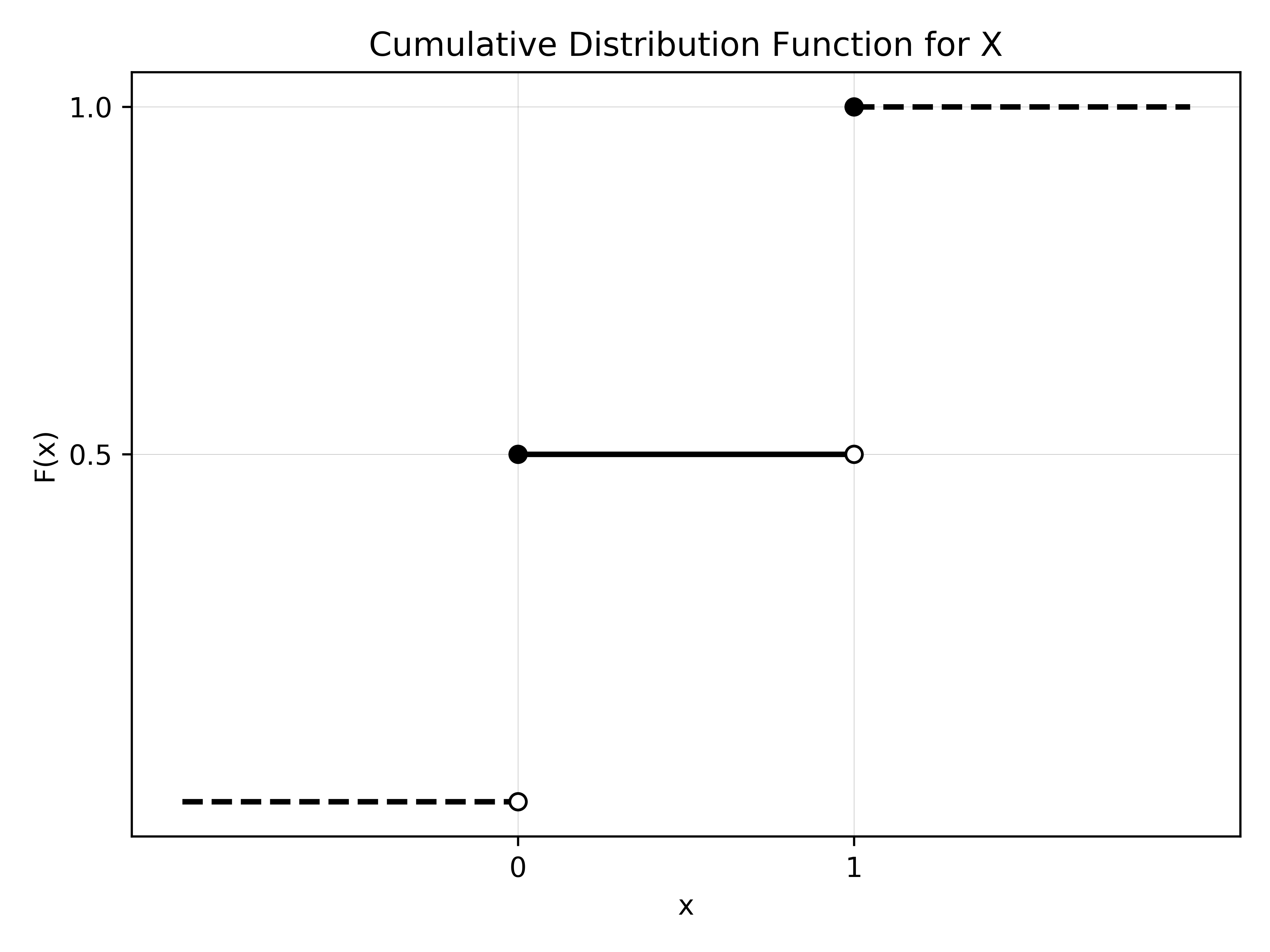
2. Plot it, ‘et voilá’, we’ve our graphic for the Bernoulli’s cumulative distribution function.

bernoulli.plot_cdf()

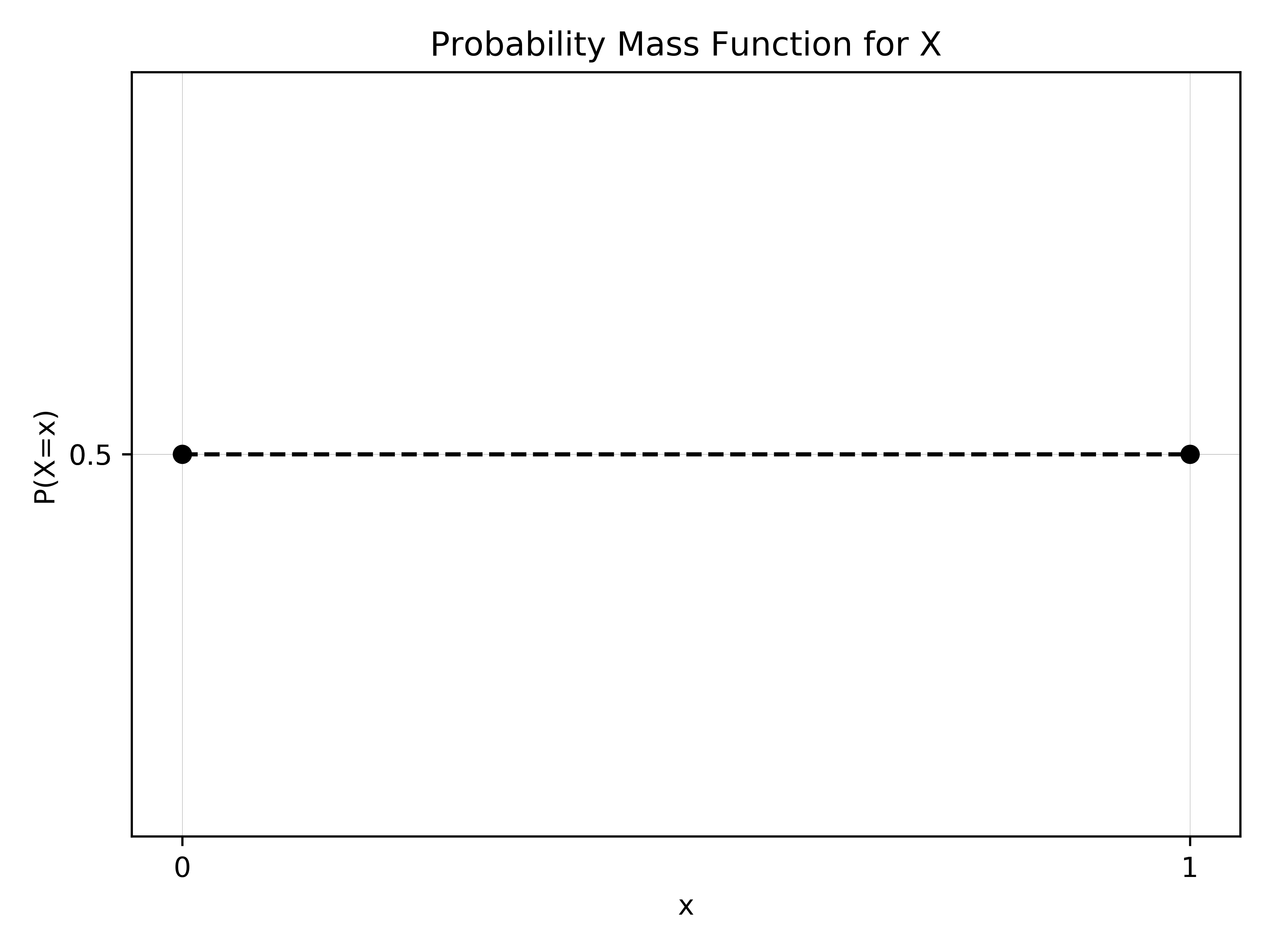
We can also plot the probability mass function

bernoulli.plot_pmf()

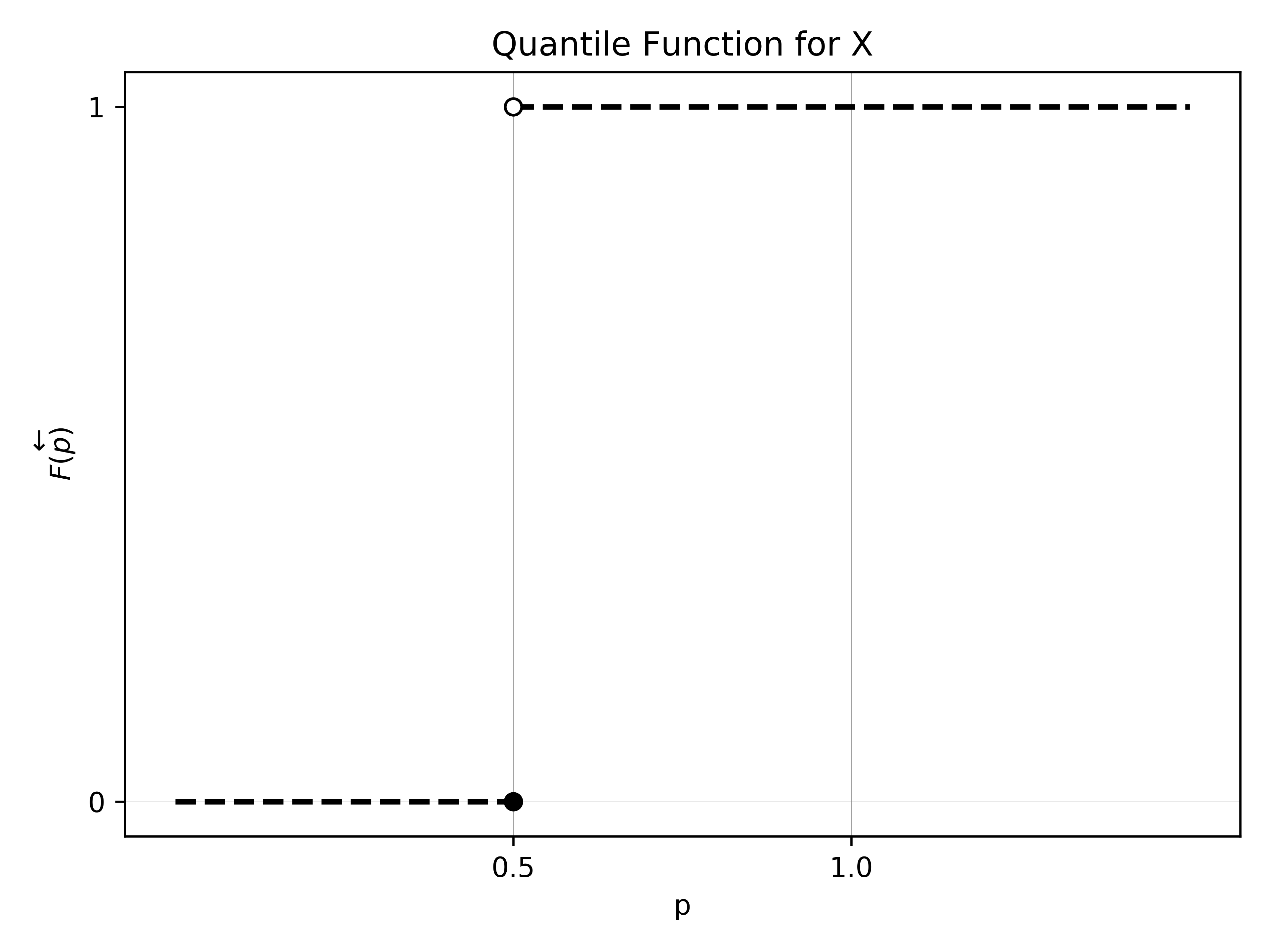
or the percentile (quantile) function

bernoulli.plot_quantile()

and you’re ready to go.

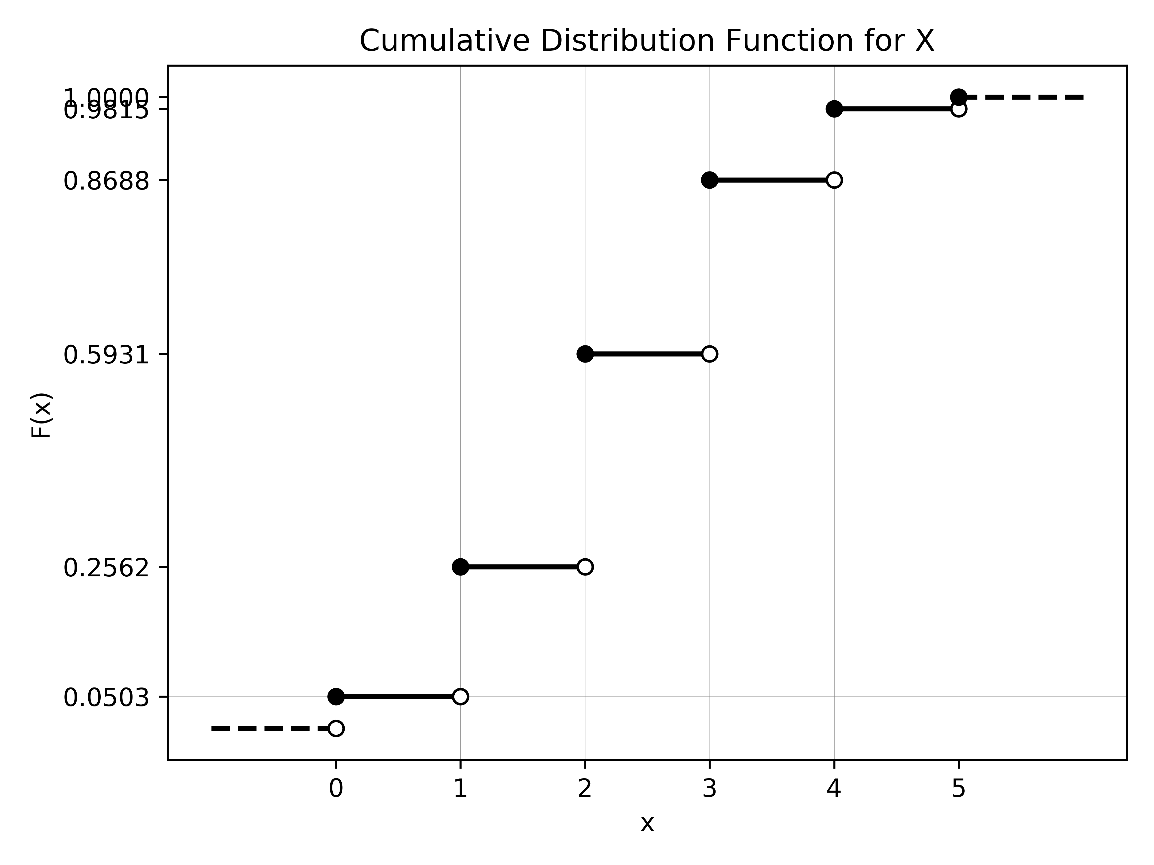
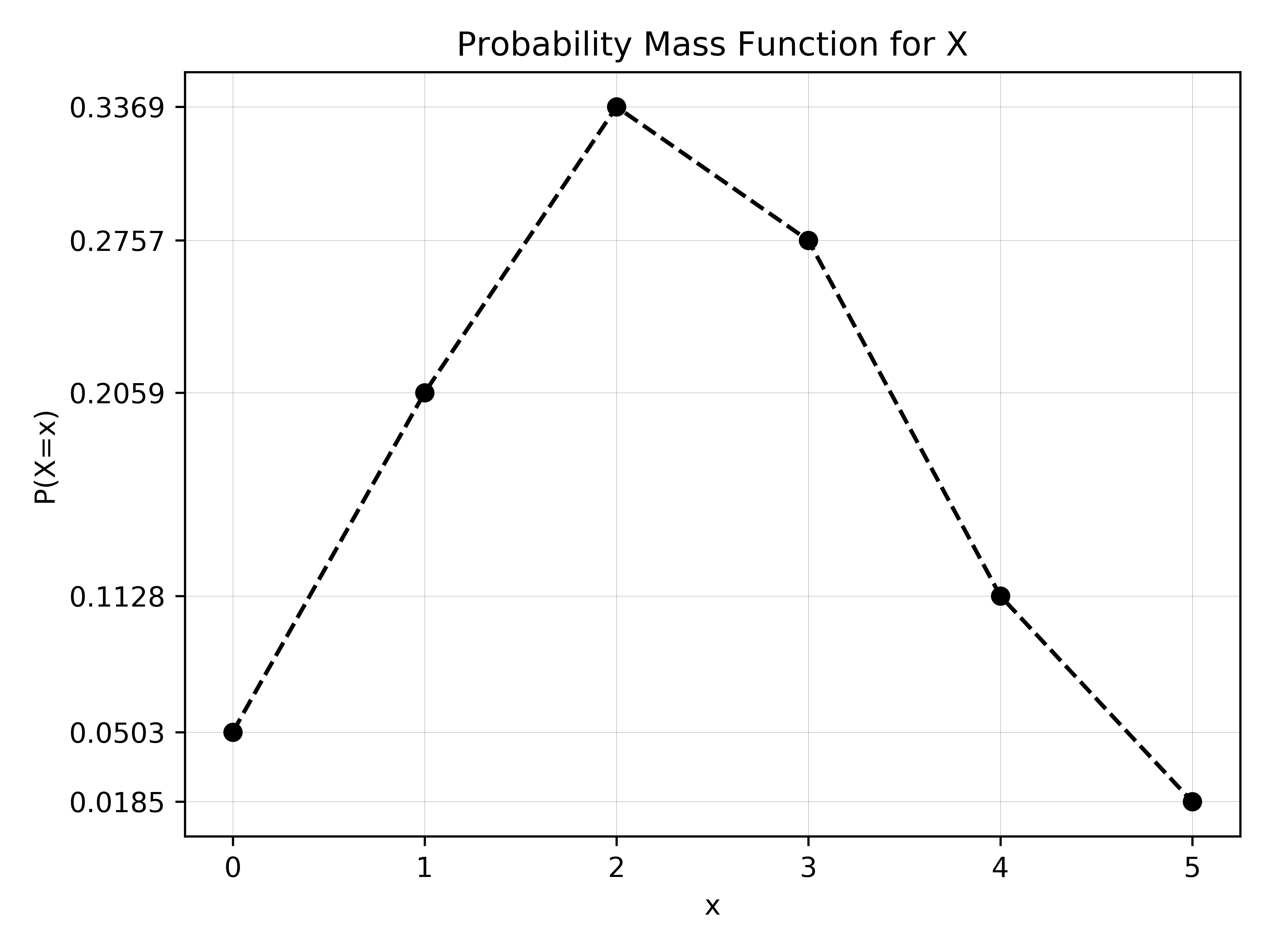
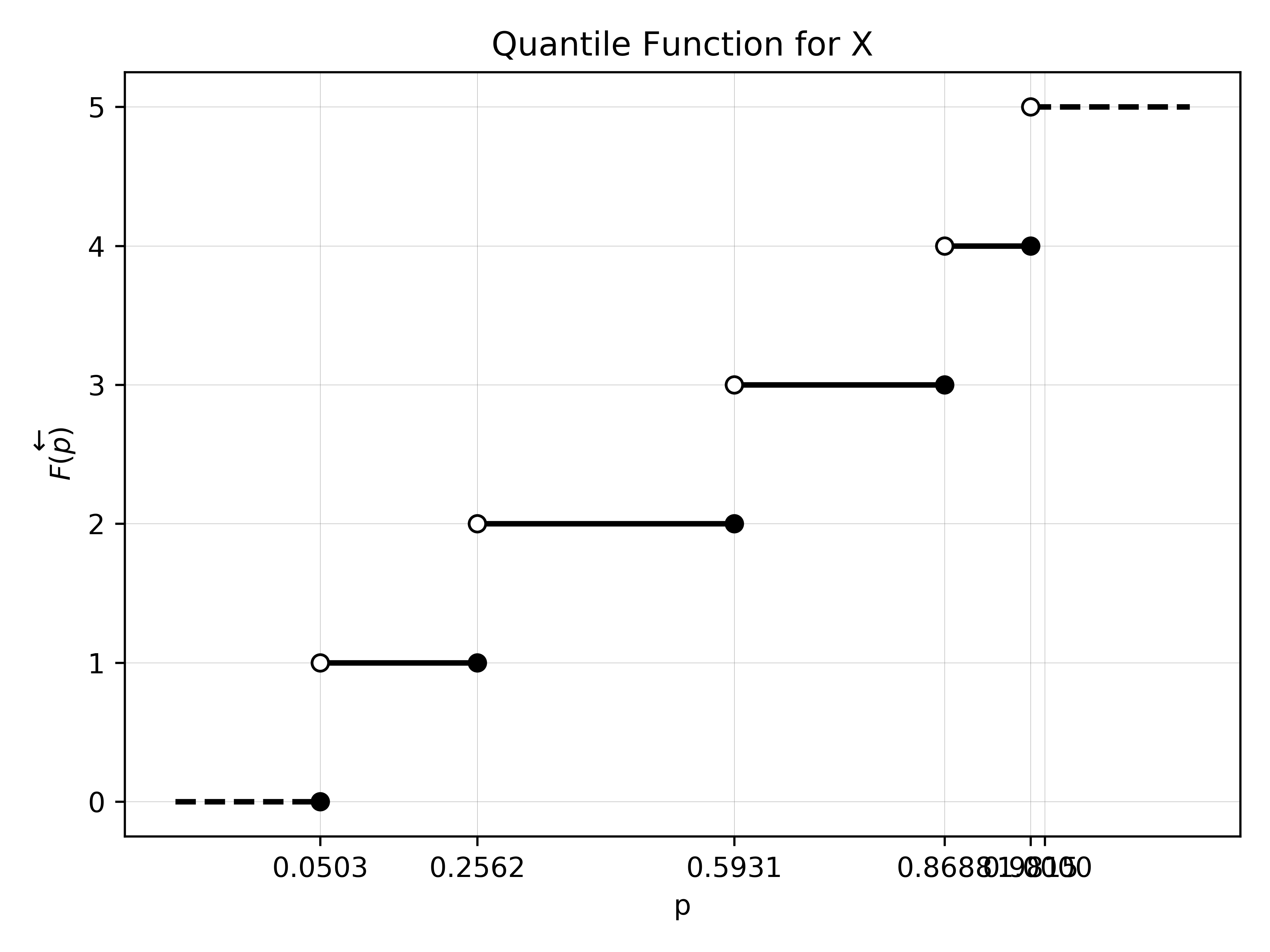
The Binomial

A simple extension of the Hello World. Consider now a Binomial; \(X\sim B(n, p)\), that is \(X\in \{0,..., n\}\) with \(P(X=x)=C^n_x p^x(1-p)^{1-x}\), with \(n \in \mathbb{N}\) and \(p \in ]0,1[\).

In this example, we’ll be plotting \(X\sim B(5, 0.5)\).

In this case we’ve as support and pmf, respectively

support=[0, 1, 2, 3, 4, 5]

prob=[0.0503284375, 0.2058890625, 0.336909375, 0.275653125, 0.1127671875, 0.0184528125].

1. Create your discrete random variable:

binomial = plot.RV(support, prob)

The result would be the same if instead of the probability mass function (pmf) you passed the cumulative distribution function (cdf).

prob=[0.0503284375, 0.2562175, 0.593126875, 0.86878, 0.9815471875, 1.0].

binomial = plot.RV(support, prob, is_pmf=False)

2. Plot the cumulative distribution function.

binomial.plot_cdf()

Plot the probability mass function

binomial.plot_pmf()

or the percentile (quantile) function

binomial.plot_quantile()

Incomplete Tails

We will use the Poisson to explain the case for an incomplete support of the random variable. Consider now a Poisson; \(X\sim P(\lambda)\), that is \(X \in \mathbb{N}_0\) with \(P(X=x)=e^{-\lambda}\frac{\lambda^x}{x!}\), with \(n \in \mathbb{N}\) and \(\lambda \in \mathbb{R}^+\).

In this case since the support is countable but not finite, we should consider that in our plot.

Incomplete Right Tail

In the example we’ll be using the \(X\sim P(5)\).

So, if we consider to plot the subset of the support [0, 1, 2, 3, 4, 5, 6, 7, 8, 9, 10, 11, 12], we are truncating the right tail. When we initialize our Poisson using the supported truncated to the right, we’ll get a warning based on the max_tol set with default 1e-12. Hence in this case, we are using

support=[0, 1, 2, 3, 4, 5, 6, 7, 8, 9]

prob=[0.006737947, 0.033689735, 0.0842243375, 0.1403738958, 0.1754673698, 0.1754673698, 0.1462228081, 0.104444863, 0.0652780393, 0.0362655774].

We should initialize our random variable stating that the right tail is incomplete, so that, the plot signs this situation, in accordance with the WARNING:root:The error of the sum of the probabilities exceeds the maximum tolerance allowed for the error. So, you should consider to mark at least one of the tails as incomplete. The error is 0.031828057306205304 with a tolerance of 1e-12.

poisson = plot.RV(support, prob, complete_right=False)

The error is due to the difference \(1-P(X\leq 9)=3.18281\%.\)

Plot the cumulative distribution function

poisson.plot_cdf()

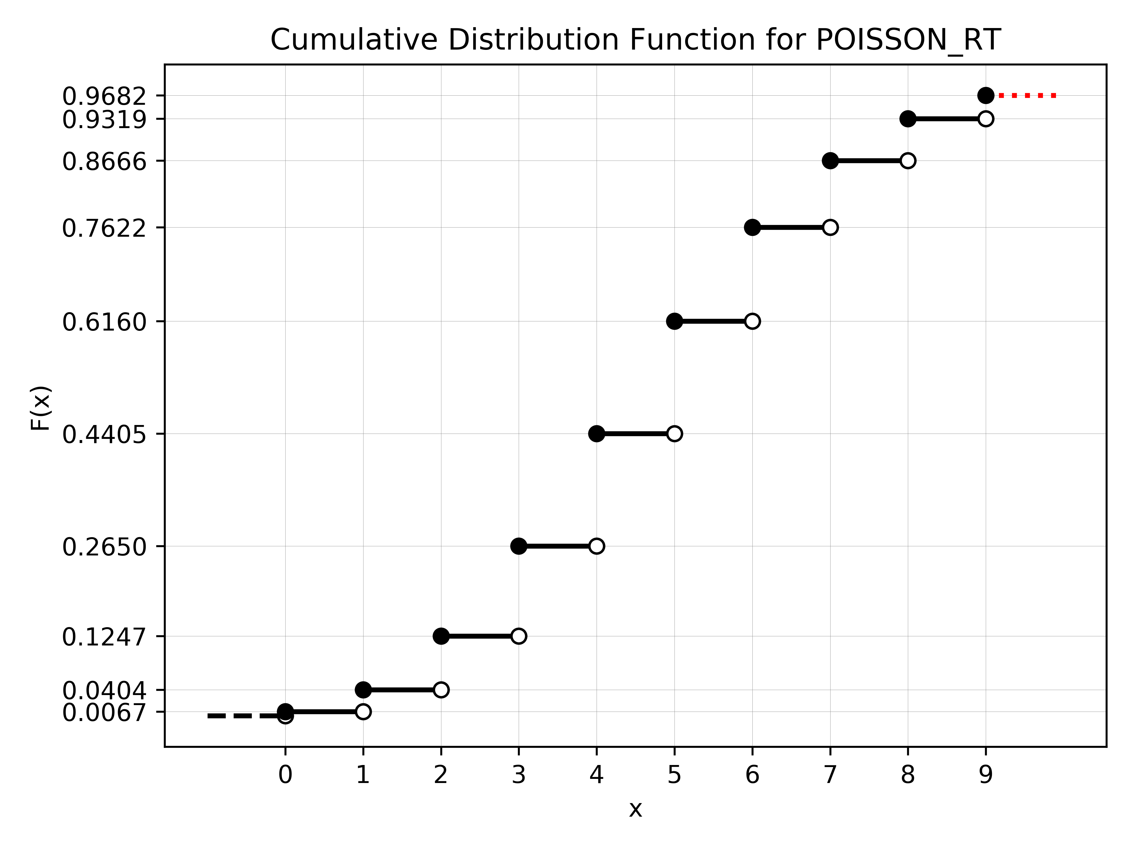
the plot, by default, marks the truncated right tail with a red dashed line.

Plot the probability mass function

poisson.plot_pmf()

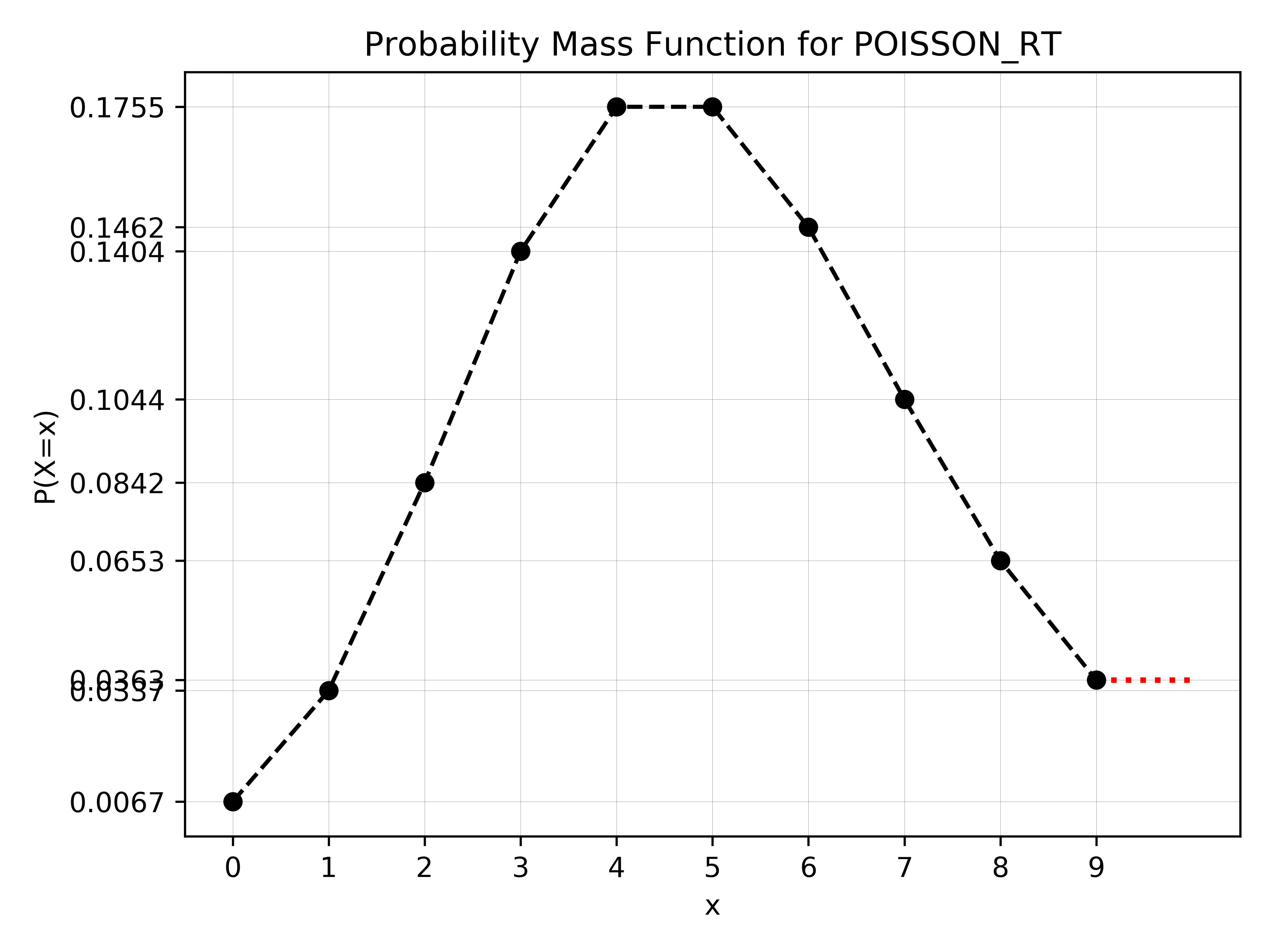
the plot, by default, marks the truncated right tail with a red dashed line.

Plot the percentile (quantile) function

poisson.plot_quantile()

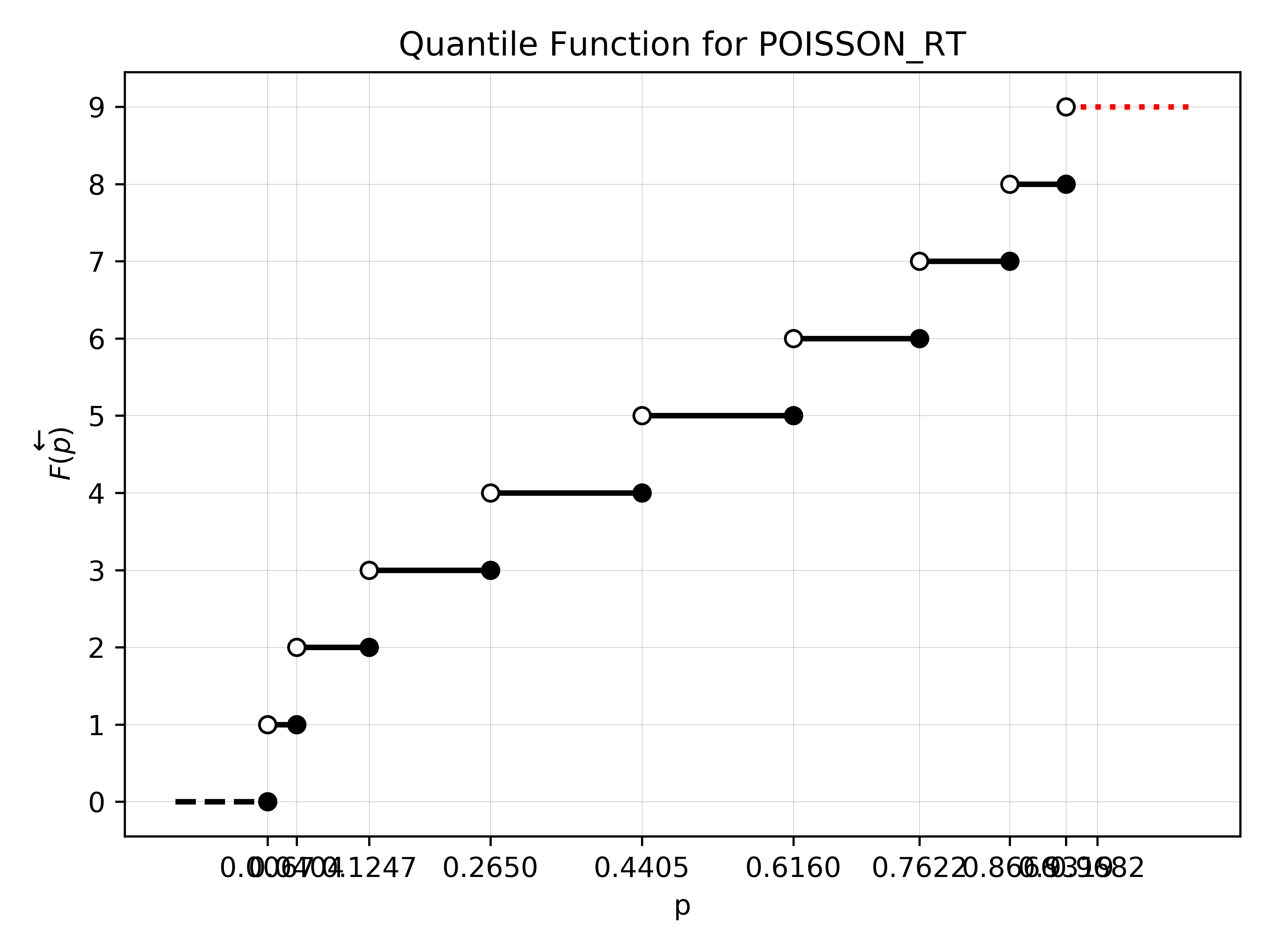
the plot, by default, marks the truncated right tail with a red dashed line.

Incomplete Left and Right Tail

In the example we’ll be using the \(X\sim P(5)\).

So, if we consider to plot the subset of the support [4, 5, 6, 7, 8, 9, 10, 11, 12], we are truncating both the left and right tails. When we initialize our Poisson using the supported truncated to the left and right, we’ll get a warning based on the max_tol set with default 1e-12. Hence in this case, we are using

support=[4, 5, 6, 7, 8, 9]

prob=[0.4404932851, 0.6159606548, 0.762183463, 0.8666283259, 0.9319063653, 0.9681719427].

So, we should initialize our random variable stating that the left and right tail are incomplete and we are using the cumulative probabilities. We’ll get a warning due to the truncation above the maximum tolerance set: WARNING:root:The error of the sum of the probabilities exceeds the maximum tolerance allowed for the error. So, you should consider to mark at least one of the tails as incomplete. The error is 0.03182805730620486 with a tolerance of 1e-12. The error is due to the difference \(1-P(X\leq 12)=3.18281\%.\)

poisson = plot.RV(support, prob, is_pmf=False, complete_left=False, complete_right=False)

Plot the cumulative distribution function

poisson.plot_cdf()

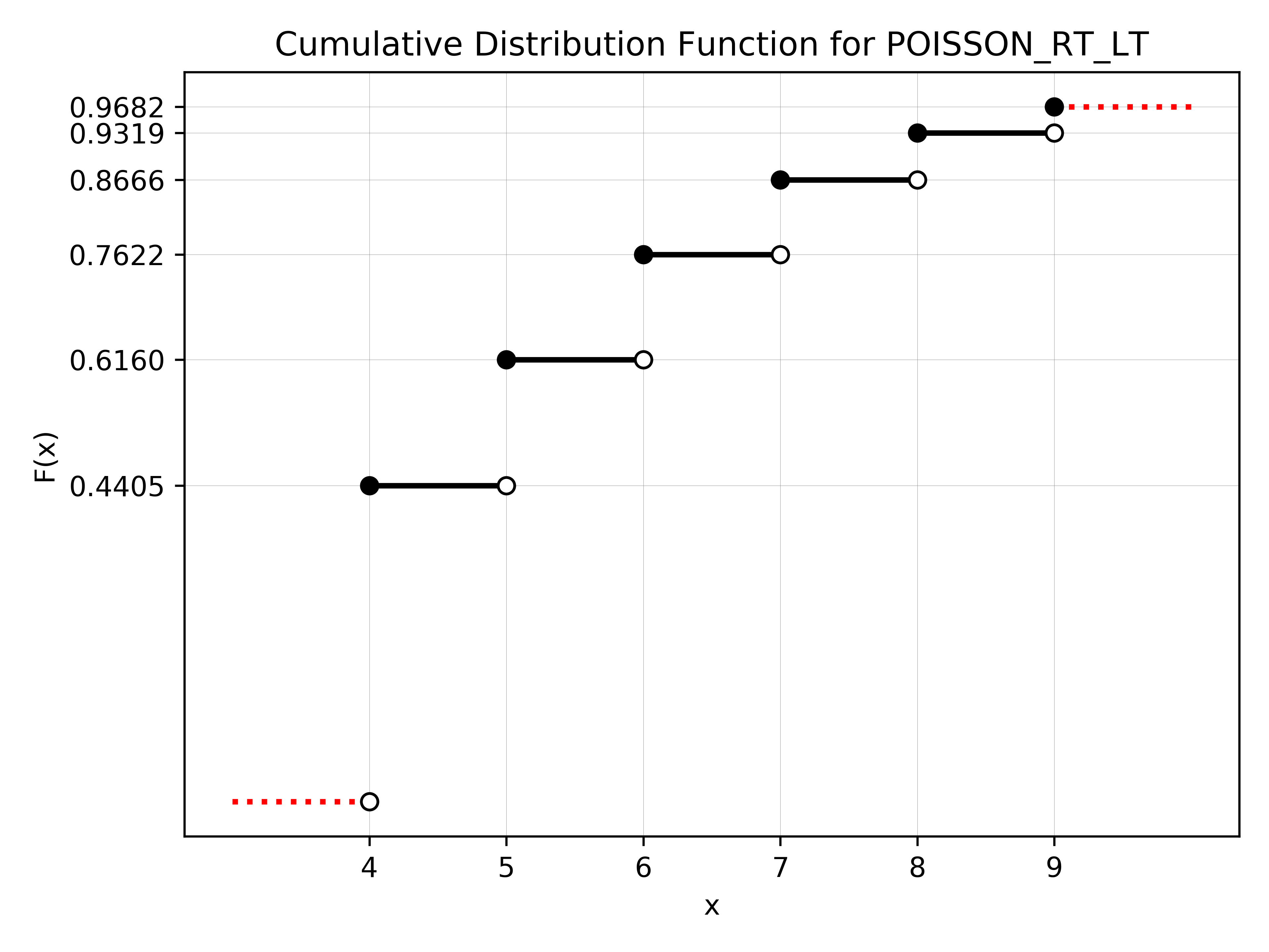
the plot, by default, marks the truncated tails with red dashed lines.

Plot the probability mass function

poisson.plot_pmf()

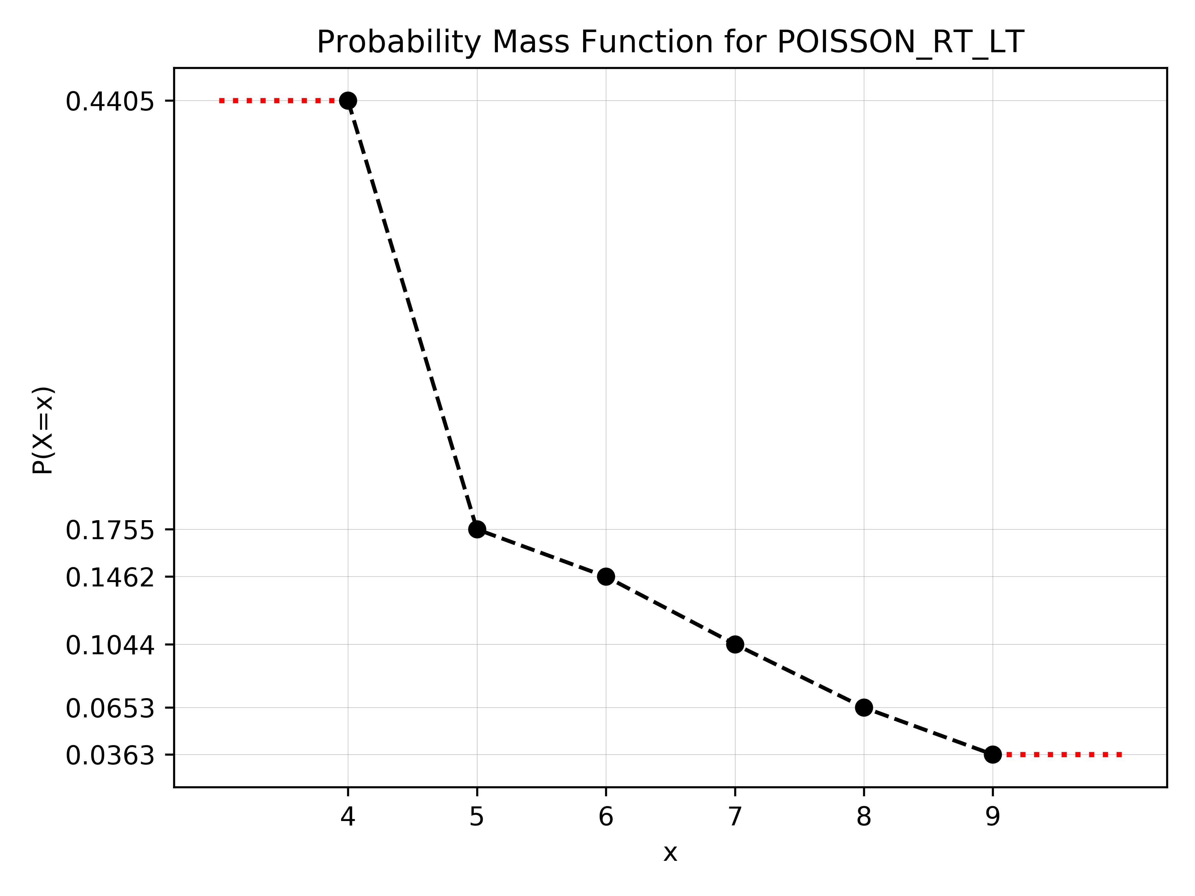
the plot, by default, marks the truncated tails with red dashed lines. Note that, in this case, the plotted probability of the smallest mass point is plotted incorrectly, since we passed a truncated cumulative distribution function and we don’t have way of determining \(P(X=4)\).

Plot the percentile (quantile) function

poisson.plot_quantile()

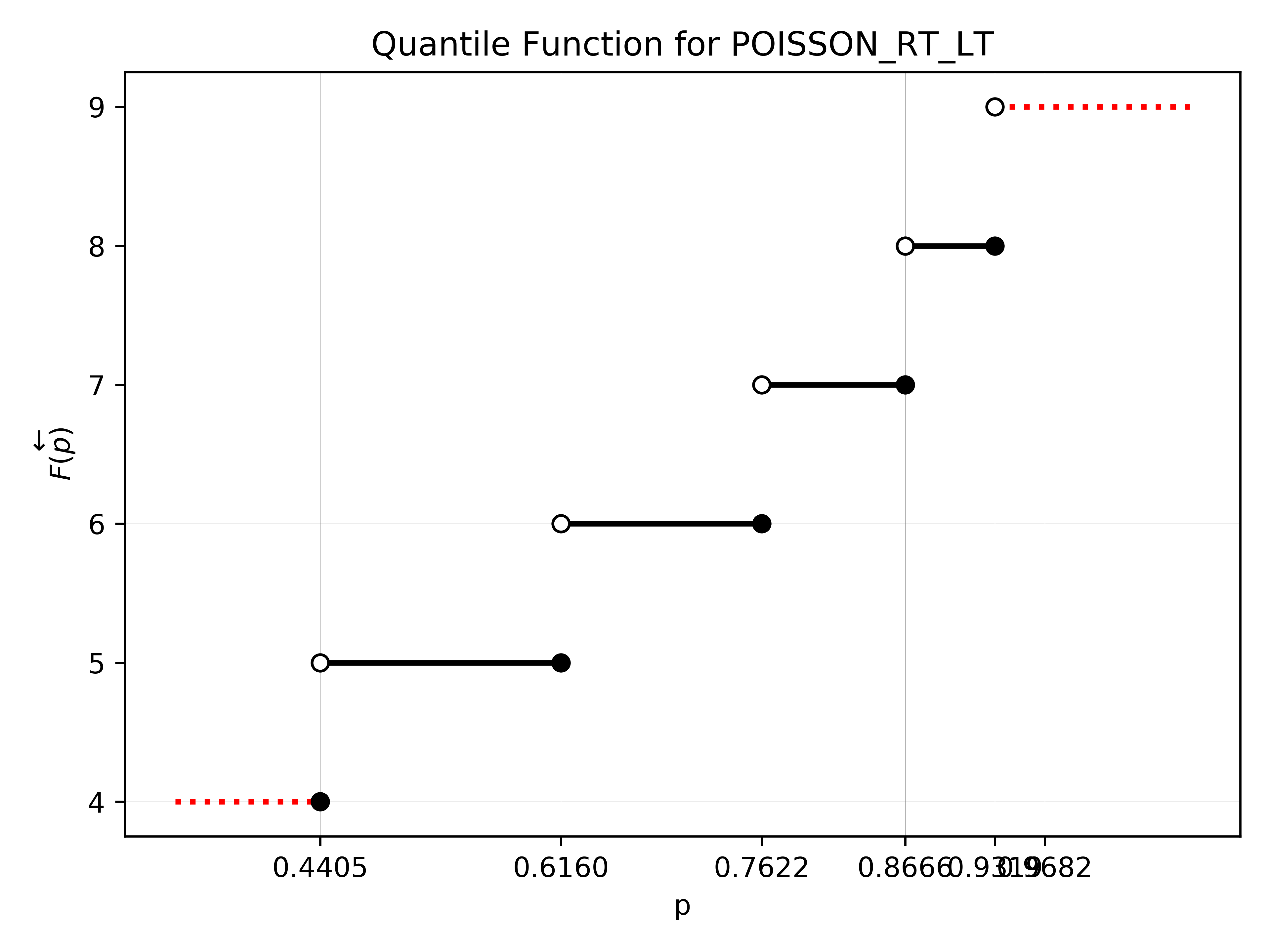
the plot, by default, marks the truncated tails with red dashed lines.